View Tab in MS Excel
View Tab

View Tab On the Home Tab, under the heading “Cells Group, Format > Unhide,” you will find the instructions that make it possible to hide and reveal worksheets. This page contains the commands that allow you to hide and reveal workbooks (as well as windows on your computer).
Sheet View
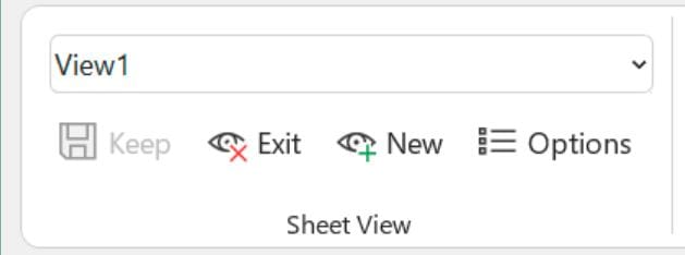
Switch Sheet View – This workbook has a drop-down list that lists all of the various sheet views that can be easily switched between (View Tab).
Keep – Creates a new sheet view that is based on the existing view in View Tab.

Exit – This function will close the sheet view that is now active and return to the default view.
New – Allows you to specify a new view for the sheet. The term “Temporary View” is used to refer to newly created views until they are saved successfully in View Tab.
Options – The only time this will be enabled is when. Displays the “Sheet View Options” dialog box, which gives you the ability to rename, duplicate, and remove individual sheets, as well as switch between multiple views in a short amount of time in View Tab.
Workbook Views
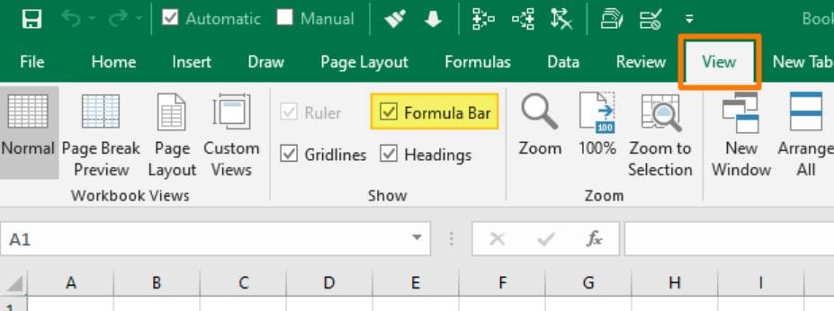
Normal – This function displays the worksheet in its standard view (View Tab). This view may also be accessed using a shortcut that is located in the bottom right corner of the status bar.
Page Break Preview – Page breaks may be adjusted using this tool. This view may also be accessed using a shortcut that is located in the bottom right corner of the status bar.

Page Layout – Presents the worksheet in the format that it will be shown on a printed page. In addition to displaying a very helpful horizontal and vertical ruler, this tool also allows you to create or edit headers and footers, check margins, row and column titles, and scale choices. The Print Preview should not be confused with this. This view may also be accessed using a shortcut that is located in the bottom right corner of the status bar.
Custom Views – Allows the “Custom Views” dialog box to be shown.
Show
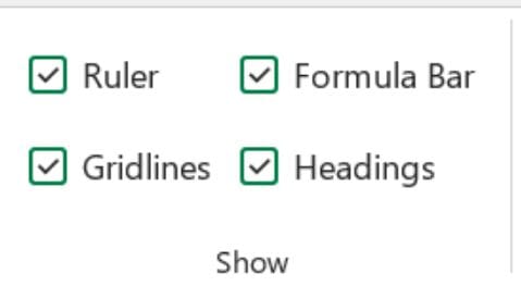
Ruler – When you are in Page Layout view, this feature will only become active. The display of the horizontal and vertical rulers may be toggled with this button. When you are in Page Layout view, you will only be able to access this feature. You have the ability to modify the units that are shown by going to the Display, Ruler Units section of the Excel Options tab. It is the default option for the ruler to show the default units that are defined in the control panel’s regional settings. Inches, centimeters, or millimeters are all alternatives for these units of measurement.

Gridlines – This toggles the display of gridlines on the worksheet that is now active. This function provides a shortcut to the Excel settings, Advanced tab, which displays settings for this worksheet and displays gridlines.
Formula Bar – Performs a toggle operation on the formula bar display. Offers a shortcut to the Excel Options menu, namely the Advanced tab and the Show formula bar.
Headings – Switches the appearance of the rows that have headings. Offers a shortcut to the Excel Options menu, namely the Advanced tab and the Show row and column headers option.
Zoom
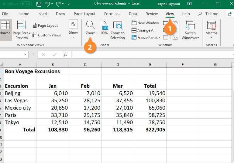
Zoom – This button brings up the “Zoom” dialog window.

100% – Resize the workbook to be one hundred percent of its regular size.
Zoom to Selection – You may zoom the worksheet so that it just shows the cells that are presently chosen.
Window
New Window – Opens a new window of the worksheet you are currently working on.
Arrange All – The screen should be tiled with all of the open windows side by side.
Freeze Panes – Turning down. Freeze Window Panes, Freeze Top Row, and Freeze First Column are the commands that may be found in the drop-down menu.
Split – Use this feature to divide the window into many panes that can be resized, giving you the ability to see the same worksheet from various perspectives.
Hide – Allows the current window or workbook to be hidden.

Unhide – This function brings up the “Unhide” dialog box, which gives you the ability to reveal a workbook or window.
View Side by Side – This will enable you to compare the contents of two different workbooks by viewing them side by side.
Synchronous Scrolling – To ensure that two windows scroll in tandem with one another, synchronize their scrolling. In order to initiate the execution of this command, it is necessary to activate the View Side by Side option.
Reset Window Position – To ensure that the two windows being compared take up an equal amount of space on the screen, reset the window positions of each of them. In order to initiate the execution of this command, it is necessary to activate the View Side by Side option.
Switch Windows – Drop-Down. The drop-down contains a list of all the workbooks/windows that are currently open.
Macros

Macros – Button that has a drop-down menu. This button is a shortcut to View Macros, which may be used to show the “Macro” dialog box, which lists all of the macros that are currently accessible. The instructions that are included in the drop-down menu are as follows: View Macros, Record Macro, and Use Relative References.
Read more:- Using of Review Tab in MS Excel (Microsoft Excel Docs). (Lession – 14)

Hi, I’m Narinder Kumar, founder of BlogsBuz.com. I create articles and generate celebrity biographies, providing verified, up-to-date content. As an SEO expert and online tools creator, I also share practical tips on making money online, finance management, blogging, and passive income. My mission is to provide accurate information and keep you away from fake content, ensuring you stay well-informed and make smart decisions online.

